In this chapter various lumped and distributed models of LDS will be formulated in both, time and transform (L or Z) domains. We will start with basic dynamic characteristics of LDS, then we will show the decomposition of dynamics to time and space components.
As a conclusion of this chapter, the accuracy of models formulated using discretization in the space domain will be analysed.
Linear deterministic models
For illustration, first assume a linear time-invariant LDS, distributed within the interval <0,L>, and time-spatial variables in an axonometric coordinate system. Results achieved will be then generalized for common types of DPS.
Further assume, provided zero initial and boundary conditions are given, that an input variable Ui(t) is fed into LDS. The output of the system will be in the form of distributed variable, Yi(x,t) – see Fig. 3.1.1.
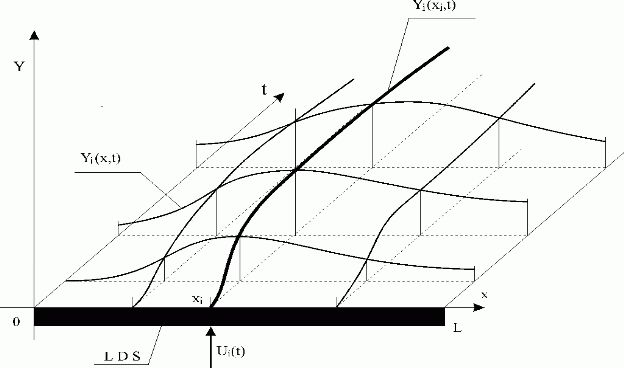
Fig. 3.1.1 LDS response to individual action of i-th input variable
| LDS | – lumped-input/distributed-output system |
| Ui(t) | – i-th lumped input variable |
| Yi(x,t) | – i-th distributed output variable |
| Yi(xi,t) | – i-th partial distributed output variable at point xi |
The relationship between these variables can be described by the convolution product:
| (3.1.1) |
where ![]() is the LDS distributed impulse response function, see Fig. 3.1.2. When Ui(t) is a unit-step (Heaviside) function in the output of LDS the distributed transient response function,
is the LDS distributed impulse response function, see Fig. 3.1.2. When Ui(t) is a unit-step (Heaviside) function in the output of LDS the distributed transient response function,  i(x,t), can be obtained.
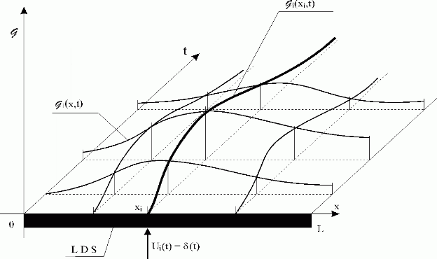
Fig. 3.1.2 LDS distributed impulse response function
| LDS | – lumped-input/distributed-output system |
Ui(t) =  (t) (t) |
– i-th lumped input, unit impulse (Dirac) (t)-function |
 i(x,t) i(x,t) |
– i-th distributed impulse response function |
| i(xi,t) |
– i-th partial distributed impulse response function at point xi |
Similarly, it is possible to get relationships between the individual input variables ![]() and the corresponding distributed output variables
and the corresponding distributed output variables ![]() .
.
The resulting distributed output variable can be then expresed by the equation
| (3.1.2) |
Now, choose measurement points with coordinates x1,…,xi,…,xn near to input points of the control variables, U1(t),…,Ui(t),…,Un(t) feeding. At these points, an ideal measurement process can be assumed, without any distortion of measured variables. At these points, on individual surfaces Y1(x,t),…,Yi(x,t),…,Yn(x,t) partial distributed outputs – curves Y1(x1,t),…,Yi(xi,t),…,Yn(xn,t) – are obtained – see Fig. 3.1.3.
Further, at points x1,…,xi,…,xn and on surfaces of individual distributed impulse response functions, partial distributed impulse response functions ![]() ,…,
,…,![]() ,…,
,…,![]() , Fig. 3.1.2, can be found.
, Fig. 3.1.2, can be found.
Using relationship (3.1.1), it yields:
| (3.1.3) | |
| (3.1.4) | |
| (3.1.5) |
See Fig. 3.1.3.
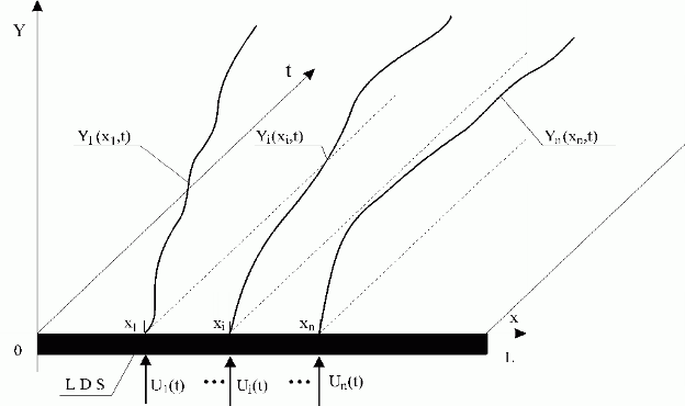
Fig. 3.1.3 Partial distributed output variables at measurement points
x1,.., xi,.., xn
| LDS | – lumped-input/distributed-output system |
| U1(t),…,Ui(t),…,Un(t) | – lumped input variables |
| Y1(x1,t),…,Yi(xi,t),…,Yn(xn,t) | – partial distributed output variables at points x1,…,xi,…,xn |
Assuming discrete input variables and zero-order hold units, {Hi}i . Discrete models can be expressed, similarly, in the form of the convolution summation:
| (3.1.6) |
where ![]() is distributed impulse response function of LDS with zero-order hold unit, Hi: HLDS.
is distributed impulse response function of LDS with zero-order hold unit, Hi: HLDS.
For simplicity, assume further T = 1 and  = 0. Hence eq. (3.1.6) gives:
| (3.1.7) |
See Fig. 3.1.4. When zero-order hold units, {Hi }i are used, the distributed discrete impulse response functions for t = k can be obtained as follows
| (3.1.8) |
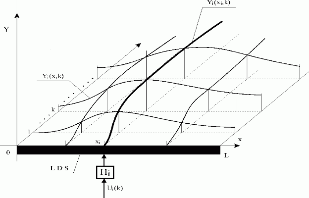
Fig. 3.1.4 Influence of the Ui(k) sequence on LDS with hold unit Hi
| LDS | – lumped-input/distributed-output system |
| Hi | – zero-order hold unit |
| Ui(k) | – i-th input sequence |
| Yi(x,k) | – i-th distributed output variable |
| Yi(xi,k) | – i-th partial distributed output variable at point xi |
Then the overall distributed output variable of LDS and {Hi }i: HLDS can be expressed in the form:
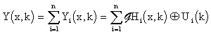 |
(3.1.9) |
Hereinafter, the lumped and distributed variables will be mostly assumed to be defined in discrete time instants. When reguired, distributed disturbances and output variable of HLDS block will be assumed as continuous signals, Figs. 3.1.5, 5.2.1, 5.2.2, etc.
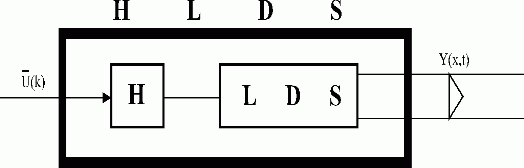
Fig. 3.1.5 HLDS output variable
| LDS | – lumped-input/distributed-output system |
| H | – block of zero-order hold units {Hi }i |
| Y(x,t) | – continuous distributed output variable |
| – vector of lumped input variables |
For points x1,…,xi,…,xn located in surroundings of lumped input variables feeding, partial distributed output variables, Y1(x1,k),…,Yi(xi,k),…,Yn(xn,k) or partial distributed impulse response functions, H1(x1,k),…,Hi(xi,k),…,Hn(xn,k) can be obtained.
Then the following convolution summations hold true:
| (3.1.10) | |
| (3.1.11) | |
| (3.1.12) |
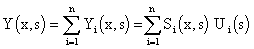
Operating in s or z domain, we get the relations:
| (3.1.13) | |
 |
(3.1.14) |
| (3.1.15) | |
| (3.1.16) | |
| (3.1.17) |
where {Si(x,s)}i and S1(x1,s),…,Si(xi,s),…,Sn(xn,s) are the respective transfer functions.
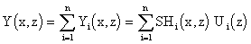
Further, it holds
| (3.1.18) | |
 |
(3.1.19) |
| (3.1.20) | |
| (3.1.21) | |
| (3.1.22) |
where {SHi(x,z)}i, resp. SH1(x1,z),…,SHi(xi,z),…,SHn(xn,z) are transfer functions of the distributed system under consideration assuming zero-order hold units.
This approach allows to associate LDS and zero-order hold units {Hi}i: HLDS with distributed and lumped blocks as shown in Figs. 3.1.6 – 8.
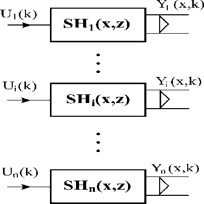
Fig. 3.1.6 Distributed systems associated with HLDS
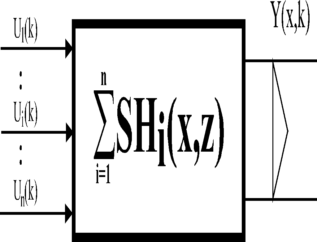
Fig. 3.1.7 HLDS model
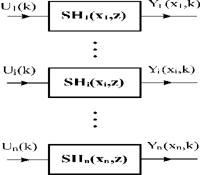
Fig. 3.1.8 Lumped systems associated with HLDS
When the vector of lumped variables, {Ui(k)}i , operates as input of the block HLDS, the overall output variable, Y(x,k) is obtained. Let us associate lumped and distributed components with this distributed variable by means of introduced lumped and distributed systems.
When the vector of {Ui(k)}i is entering at points x1,…,xi,…,xn , in outputs of blocks SH1(x1,z),…, SHi(xi,z),…, SHn(xn,z) partial distributed output variables Y1(x1,k),…,Yi(xi,k),…,Yn(xn,k) are generated. Distributed output variables from blocks SH1(x,z),…,SHi(x,z),…,SHn(x,z): Y1(x,k),…, Yi(x,k),…,Yn(x,k) „slide„ on these trajectories – see Fig. 3.1.9.
Hence, the overall output variable is given by the relationship:
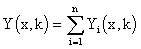
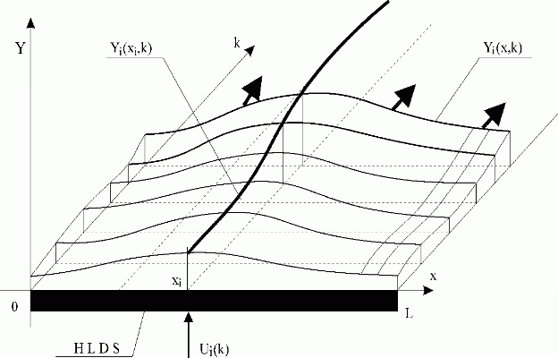
Fig. 3.1.9 Yi(x,k) „ sliding“ on trajectory Yi(xi,k)
| HLDS | – lumped-input/distributed-output system with zero-order hold units |
| Ui(k) | – i-th lumped input variable |
| Yi(xi,k) | – i-th partial distributed output variable |
| Yi(x,k) | – i-th distributed output variable |
 |
– sliding direction |
When the discrete representation is considered, the distributed system dynamics is given by the set of discrete distributed impulse response functions, ![]() .
Let us introduce on this set the reduced characteristics in the following form:
.
Let us introduce on this set the reduced characteristics in the following form:
 |
(3.1.23) |
 |
(3.1.24) |
 |
(3.1.25) |
Some reduced characteristics are shown in Fig. 3.1.10.
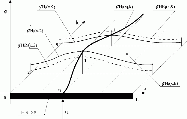
Fig. 3.1.10 Partial reduced discrete impulse responses
| HLDS | – lumped-input/distributed-output system with zero-order hold units |
| – i-th distributed impulse response function | |
| – i-th partial distributed discrete impulse response function at point xi, along time k | |
| – i-th partial distributed discrete impulse response functions in the direction x | |
| – i-th reduced partial distributed discrete impulse response functions in the direction x |
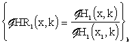
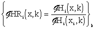
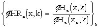
Using the reduced functions, eq. (3.1.7) yields:
| (3.1.26) | |
| (3.1.27) | |
| (3.1.28) |
For xi e.g. eq. (3.1.27) gives
| (3.1.29) |
since HRi(xi,k) = 1.
It means that Hi(xi,k) determines the partial distributed output variable in the time domain at point xi. See Fig. 3.1.11.
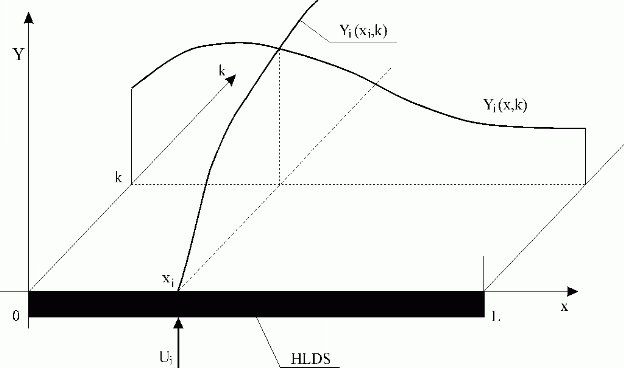
Fig. 3.1.11 Distributed output variable in time and space domains
| HLDS | – lumped-input/distributed-output system with zero-order hold units |
| Ui | – i-th lumped input variable |
| Yi(xi,k) | – i-th partial distributed output variable in the time domain |
| Yi(x,k) | – i-th partial distributed output variable in the space domain |
The distributed output variable in the space domain at a point k is given again by linear combination of reduced dynamic characteristics, {HRi(x,k)}i,k according to eq. (3.1.26-28).
Following this approach, the dynamics of the object under consideration is decomposed to
– time components
| {Hi(xi,k)}i,k |
(3.1.30) |
for i, xi chosen – variable k
– space components
| {HRi(x,k)}i,k |
(3.1.31) |
for i, k chosen – variable x.
Now let us analyse the decomposition of the distributed output variable and dynamic characteristics in steady-state.
The steady-state of distributed output variable, Y(x, ), can be expressed using steady-state distributed transient response functions:
 ![]() , where
, where ![]() are the transient responses of HLDS to unit-step functions, 1(k), at each input,
are the transient responses of HLDS to unit-step functions, 1(k), at each input, ![]() , Fig. 3.1.12.
, Fig. 3.1.12.
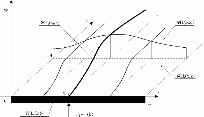
Fig. 3.1.12 i-th distributed transient response of HLDS
| HLDS | – lumped-input/distributed-output system with zero-order hold units |
| Ui = 1(k) | – i-th lumped input variable, discrete unit-step function |
| – i-th distributed transient response | |
| – i-th distributed transient response at a time q | |
| – i-th partial distributed transient response at a point xi |
Now, introduce reduced steady-state distributed transient responses at a time k – Fig. 3.1.13 – in the form:
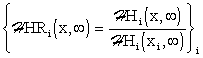 |
(3.1.32) |
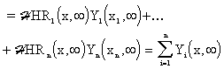
Then
| (3.1.33) | |
| (3.1.34) | |
| (3.1.35) |
See Fig. 3.1.14, where
| (3.1.36) | |
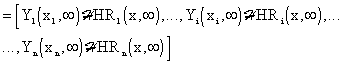 |
(3.1.37) |
In this limit case, the dynamics of the object under consideration in steady-state is split into
– time components
| (3.1.38) |
– space components
| (3.1.39) |
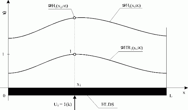
Fig. 3.1.13 i-th steady-state distributed transient response and reduced transient response
| HLDS | – lumped-input/distributed-output system with zero-order hold units |
| – i-th steady-state distributed transient response | |
| – i-th steady-state distributed reduced transient response | |
| Ui = 1(k) | – i-th lumped input variable, discrete unit-step function |
Fig. 3.1.14 ![]()
| HLDS | – lumped-input/distributed-output system with zero-order hold units |
| {Ui()}i |
– steady-state lumped input variables |
| Y(x,) |
– overall distributed output variable |
 |
|
| Y1(x1,),…,Yi(xi,),..,Yn(xn,) |
– lumped output variables, partial distributed output variables in points x1,…,xi,…,xn respectively |
| {HRi(x,
)}i=1,n |
– steady-states of the distributed reduced transient responses |
In control the further decomposition of the distributed system dynamics will be frequently used
– time components
| (3.1.40) |
– space components
| {HRi(x,
)}i |
(3.1.41) |
Model accuracy
In modeling of LDS, discretization in both, time and space domain, similarly as in numerical solutions of PDE or FEM, will be used . The distributed output variable will be calculated or measured at points appropriately chosen within an interval <0,L>, in the form of discrete values. In other points of this interval, values of distributed output variable will be fitted using appropriate interpolations methods.
Let us select the following points for spatial discretization from the above interval
{0=x1,..,xi,..,xj,…,xn,…,xm=L}
Notice that the above points are, in general, different from the ones selected for measurement in the neighbourhood of actuating inputs.
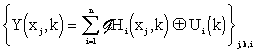
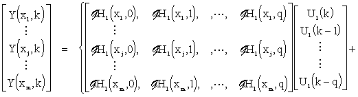
Now let us carry out spatial discretization of the discrete-time model, having lumped-input distributed-output – eq. (3.1.9). Then at points {xj}j=1,m chosen we have
 |
(3.2.1) |
or in a vector form
| (3.2.2) |
where {Ui(k)}i,k are sequences of HLDS input variables and {Hi(xj,k)}i,j,k represent the values of discrete distributed impulse response functions. Assume, that for particular i, j and r > q, the following relationship holds true: Hi(xj,r) = 0, Fig. 3.2.1. Where q denotes the LDS settling time.
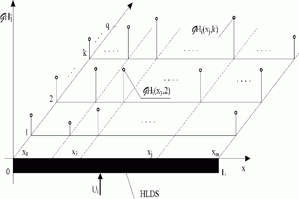
Fig. 3.2.1 Values of i-th distributed impulse response function at points {xj}j=1,m
| HLDS | – lumped-input/distributed-output system with zero-order hold units |
| Ui | – i-th lumped input variable |
| – values of i-th discrete distributed impulse response function after discretization in space domain |
Eq. (3.2.2) can be rewritten into the form:
 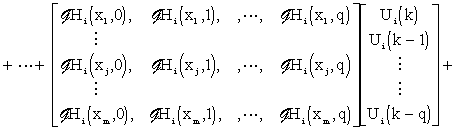 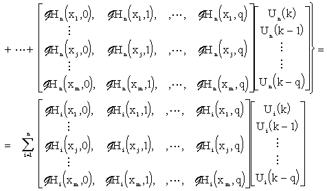 |
(3.2.3) |
Here, particular matrices correspond to distributed discrete impulse response functions of the system under consideration, see Fig. 3.2.1.
Values of distributed output variable at other points of the interval <0,L> can be obtained by interpolation methods through spline functions. The approximation procedure is to be chosen with respect to the desired accuracy. Therefore in further no separate distinction will be made between approximates and approximated variables.
In further presented results will be exploited at optimal design of DPS. Therefore, the reader interested mainly in modeling and control area can skip the rest and continue with next chapter.
The accuracy of the model constructed is ensured by standard methods of numerical mathematics. As an illustration, let us now analyse the accuracy of the model in the neigbourhood of the steady-state distributed output variable, e.g. of Y(x,), see Fig. 3.1.14.
Differential properties of Y(x,) will be evaluated using modulus of continuity and higher order derivative norms in appropriate functional spaces [22, 53, 54, 75, 83]:
| (3.2.4) |
for h  L
L
| (3.2.5) | |
| (3.2.6) |
In the interpolation using cubic spline functions, provided uniform displacement of approximation nodes is assumed, the deviations between distributed variable, Y(x,), and its approximation, Ya(x,), are less than maximal values presented in Tab. 3.1. These values were determined in the theory of spline functions, e.g. Y. S. Zavialov et. al. [83].
Tab. 3.1 Deviations between Y(x,
) and Ya(x,)
| Classes of approximated functions Y(x,) |
Maximal values of deviations between functions Y(x,) and Ya(x, ) |
 |
– net of approximating nodes in the interval <0,L>: 0 = x1 <… < xi < xi+1 <… < xm = L, length of an interval <xi, xi+1>: xi+1 – xi = h |
 |
– modulus of continuity |
| Ck<0,L> | – class of functions with k-th order continuous derivatives |
| – class of functions f(x) in interval <0,L>, whose elements have n-1 degree continuous derivatives and n-th derivatives are from space LP<0,L>, 1 p |
|
– n > k is a class of functions, f(x), where: f(x) Ck<0,L> and f(x)Cn<xi,xi+1>, i=1,2,….,m-1 Ck<0,L> and f(x)Cn<xi,xi+1>, i=1,2,….,m-1 |
|
| – n > k, 1 p is a class of functions, f(x), where: f(x)Ck<0,L> and f(x)
|
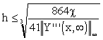
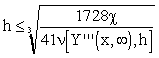
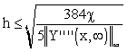
For a model accuracy specified, it is possible to determine backward the equidistant displacement of approximation nodes in an interval <0,L> for calculating and measuring the discrete values, {Y(xj,)}j of the distributed output variable.
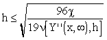
For example, from the second row of Tab. 3.1, for a desired model accuracy ,  , it comes:
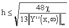 |
(3.2.7) |
The greatest value of h, satisfying the above inequality is assumed, whose integer multiple is L. In such a way, Tab. 3.1 can be transformed into Tab. 3.2.
It is known, that in approximations using spline functions a significant reduction of the number of nodes can be achieved by their non-equidistant location. For given Y(x,) and accuracy, , specified, an adequate model can be fit by minimization of the deviations norm ![]() chosen with respect to non-equidistant distribution of the nodes. This model describes changes of the distributed output variable in neighbourhood of Y(x,) with the accuracy requested, assuming minimal number of discrete values, {Y(xj,
)}j of the distributed output variable. Hence, the model of minimal complexity is fit.
chosen with respect to non-equidistant distribution of the nodes. This model describes changes of the distributed output variable in neighbourhood of Y(x,) with the accuracy requested, assuming minimal number of discrete values, {Y(xj,
)}j of the distributed output variable. Hence, the model of minimal complexity is fit.
Tab. 3.2 Maximal distances of approximation nodes for requested
| Classes of approximated functions Y(x,) |
Maximal distances of approximations nodes h |
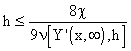 |
|
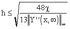 |
|
 |
|
 |
|
 |
|
 |
The approximated distributed output variable using spline approximation is then got in the form:
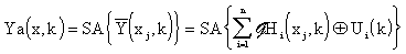 |
(3.2.8) |
where SA stands for spline approximation.
For accuracy prescribed,
, Fig. 3.2.2, the distributed output variable, Y(x,k), and its approximation, Ya(x,k), determine in a fully equivalent way the changes of the distributed output. Therefore, in accordance with conventions used in the domain of numerical solutions of PDE and FEM, no difference will be made, hereinafter, between approximates and approximated variables. Therefore Y(x,k) will stand for the model output in general.
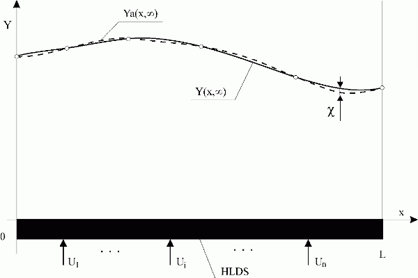
Fig. 3.2.2 Equivalence of Y(x,) and Ya(x,) for given
| HLDS | – lumped-input/distributed-output system with zero-order hold units |
| {Ui}i | – lumped input variables |
| Y(x,)/Ya(x,) |
– distributed output variable and its approximation in steady-state |
|
– accuracy of the approximation |
| <<< Previous | Next >>> |