In this chapter, possible approaches to LDS analytical and experimental identification will be analysed. In analytical identification, standard forms of differential equations and FEM will be used to fit models of the systems under consideration.
In experimental identification, methods of lumped system experimental identification and approximation methods using spline functions in spatial domain will be exploited. As a conclusion of this chapter, ways of model construction with respect to the accuracy requested will be discussed.
Analytical identification
In analytical identification physical principles are used. Mathematical models in the form of ordinary differential equations will be associated with actuating members of lumped input variables, {SAi}i. Mathematical models in the form of partial differential equations will be associated with distributed input generators, {GUi}i , and with distributed-input/distributed-output system – see Figs. 2.2, 4.1.2.
These equations, with initial and boundary conditions given, will be further transformed to standard forms and associated with lumped and distributed impulse response functions – Green’s functions [9,10]. This procedure allows to determine distributed impulse response functions of lumped-input/distributed-output system to be identified.
Assume Green’s functions in the following common forms:
| (4.1.1) | |
| (4.1.2) | |
| (4.1.3) |
Then the LDS distributed impulse response functions will take the form:
 |
(4.1.4) |
The dynamics of distributed input generators can be modeled in the form:
| (4.1.5) |
where functions {Ti(x)}i, shaping units in the space domain, in intervals {<xi1, xi2>}i  <0,L>, represent space components of the distributed input generators’ dynamic responses, {GUi}i . Fig. 4.1.1. Time components of the responses are represented by impulse response functions, {gGUi(t,
  )}i. Therefore:
 |
(4.1.6) |
see Fig. 4.1.2.
Such standard forms have been formulated, in principle, for all ordinary and partial differential equations. For example, in A. G. Butkovskiy’s monograph cited above, practically all the engineering interesting standard forms of ordinary and partial differential equations have been presented with more than 500 boundary value problems. Transfer functions of individual standard forms can be also found there enabling to formulate lumped-input/distributed-output models in the form of distributed transfer functions – see Fig. 4.1.2.
Assign the following transfer functions to subsystems of lumped-input/distributed-output systems :
| (4.1.7) | |
| (4.1.8) | |
| (4.1.9) |
Transfer functions between {Ui(s)}i and {Yi(x, s)}i then will have the form:
 |
(4.1.10) |
If
| (4.1.11) |
then
 |
(4.1.12) |
see Fig. 4.1.2.
This brief analysis shows that all the available results of analytical modeling of lumped and distributed systems can be utilized as well in analytical identification of the LDS.
As an illustration, we will demonstrate herein some differential equations in the role of lumped and/or distributed models based upon references [9, 10]. For simplicity we shall present the mathematical models as Model 1,…
Fig. 4.1.1 Various forms of functions Ti(x), representing the space component of the distributed input ( GUi ) generator dynamics
| DDS | – distributed-input/distributed-output system |
| <xi1,xi2> | – shaping interval in the space domain |
| a) | – triangular form of Ti(x), shaping unit in the space domain |
| b) | – sinusoidal form of Ti(x), shaping unit in the space domain |
| c) | – constant form of Ti(x), shaping unit in the space domain |
| d) | – arbitrary form of Ti(x), shaping unit in the space domain |
Fig. 4.1.2 LDS transfer functions
| {SAi}/{SAi(s)}i | – actuating members and their transfer functions |
| {SGi}/{SGi(s)Ti}i | – generators of distributed input variables and their transfer functions |
| {SGi(s)}i | – transfer functions in time domain |
| – shaping units in space domain | |
DDS/S(x, ,s) ,s) |
– distributed-input/distributed-output system and its transfer function |
Model 1
| (4.1.13) | |
Standardizing function:
| (4.1.14) |
Green’s function:
| (4.1.15) |
Transfer function:
| (4.1.16) |
Then the output variable is given in the form of convolution product of the standardizing and Green’s functions:
 |
(4.1.17) |
Model 2
| (4.1.18) | |
| (4.1.19) | |
| (4.1.20) |
where ![]()
| (4.1.21) |
Model 3
| (4.1.22) | |
 |
(4.1.23) |
 |
(4.1.24) |
where
 |
and ![]() are linear independent solutions of homogenous differential equation (4.1.22). Vk can be got by the substitution of the k-th column of the determinant V by vector [0, 0, …, 0, 1]. Further:
are linear independent solutions of homogenous differential equation (4.1.22). Vk can be got by the substitution of the k-th column of the determinant V by vector [0, 0, …, 0, 1]. Further:
| (4.1.25) |
Model 4
| (4.1.26) | |
| (4.1.27) | |
 |
(4.1.28) |
 |
(4.1.29) |
Model 5
| (4.1.30) | |
 |
(4.1.31) |
| (4.1.32) | |
 |
(4.1.33) |
Model 6
 |
(4.1.34) |
 |
(4.1.35) |
 |
(4.1.36) |
 |
(4.1.37) |
Model 7
| (4.1.38) | |
 |
(4.1.39) |
| (4.1.40) | |
 |
(4.1.41) |
Using standard forms, it is possible to express very simply also the influence of initial and boundary conditions onto behavior of distributed output variable.
Let us assume the distributed input variable, having the following standard form:
| (4.1.42) |
or in the s-domain
| (4.1.43) |
where, with respect to Model 4:
U(x,t) or U(x,s) is distributed input variable
Y(x,0) = Y0(x) is initial condition
Y(0,t) = g1(t), Y(L,t) = g2(t), or g1(s), g2(s) are boundary conditions.
Since the DDS/PDE distributed transfer function is S(x,,s), then the distributed output variable, assuming the initial condition Y0(x), has the form:
 |
(4.1.44) |
considering U(x,s) = 0, g1(s) = 0 and g2(s) = 0.
The distributed output variable, with respect to the boundary conditions, takes the form
 |
(4.1.45) |
if U(x,s) = 0 and Y0(x) = 0. Applying operations with  (
( )-functions, the following relationships hold
 |
(4.1.46) |
 |
(4.1.47) |
For discrete models of LDS, matrices of respective discrete impulse response functions – Fig. 3.2.1, equation (3.2.3) – can be got from analytical models formulated in an interval <0,L>, using standard numerical methods. When more complex areas of definition are assumed, finite element method can be used. In demonstration chapter, flexible methods to calculate distributed discrete impulse response functions using MATLAB toolboxes will be shown.
As a conclusion let us note that, using eq. (4.1.45), it is also possible to associate matrices of distributed discrete impulse response functions, { Hg1(xj, k)}j,k, {Hg2(xj, k)}j,k with models according to eqs. (3.2.1, 2, 3) with boundary conditions given, as follows:
| (4.1.48) | |
| (4.1.49) |
For the overall output variable the following relationship holds:
 |
(4.1.50) |
With respect to eqs. (4.1.45), (4.1.48, 49) and assuming zero-order hold units, the input/output relations between g1(k), g2(k) and Y(x,t) can be represented by the block HgDDS, Fig . 4.1.3.
Considering unit transfer functions, {SAi(s) = SGi(s) = 1}i operate in the LDS block, Fig. 4.1.2, then for DDS input, in interval <0,L>, we get: U(x,t) =  Ui(t)Ti(x). In the LDS block, DDS with shaping units {Ti(x)}i, enabling to generate various classes of input functions, U(x,t), will remain. In such a way, a special block transforming U(x,t) to Y(x,t) is got, Fig. 4.1.4. Further, adding the block of zero-order hold units, we get the block HTiDDS, Fig. 4.1.5. This block enables to include DDS/PDE into discrete distributed parameter control system.
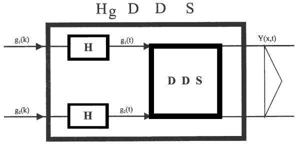
Fig. 4.1.3 Block HgDDS
| DDS | – distributed-input/distributed-output system |
| H | – zero-order hold unit |
| Y(x,t) | – distributed output variable |
| g1(t), g2(t) | – boundary conditions |
| g1(k), g2(k) | – discrete input variables |
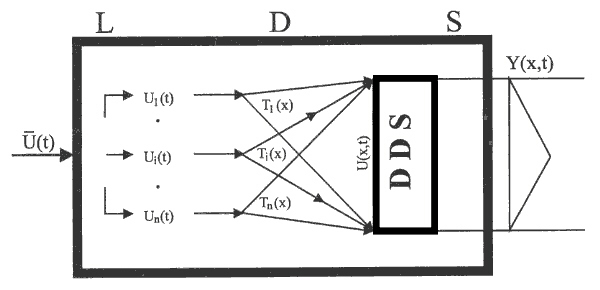
Fig. 4.1.4 DDS as special case of LDS
| LDS | – lumped-input/distributed-output system |
| DDS | – distributed-input/distributed-output system |
| {Ti(x)}i | – distributed input shaping units |
| Y(x,t) | – distributed output variable |
| U(x,t) | – distributed input variable |
| {Ui(t)}i | – lumped input variables |
| – vector of lumped input variables |
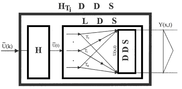
Fig. 4.1.5 Block HTiDDS
| DDS | – distributed-input/distributed-output system |
| LDS | – lumped-input/distributed-outup system |
| H | – zero-order hold units |
| {Ti}i | – distributed input shaping units |
| Y(x,t) | – distributed output variable |
| U(x,t) | – distributed input variable |
| – vector of lumped input variables |
Experimental identification
Let us consider at the output side of HLDS, the location of the measuring points in accordance with Fig. 4.2.1.
Assuming a given configuration of input/output information sources, the matrix of partial distributed discrete impulse response functions can be identified, using suitable methods – Tab. 4.2.1. Here, an ideal identification process is assumed, i.e. responses got are identical with real responses of the object being identified.
From the matrix of partial distributed discrete impulse response functions, the time components of distributed system dynamics characterisrics can be selected, see eq. (3.1.30):
| (4.2.1) |
The spatial components of the distributed controlled system dynamics characterisrics can be obtained from the partial discrete distributed impulse response functions using appropriate approximation methods.
Fig. 4.2.1 Location of the measuring points in HLDS output
| HLDS | – LDS with block of zero-order hold units |
| Ui(k) | – i-th lumped discrete input variable |
| {Y(xj,k)}j | – partial distributed output variables |
Let us consider for example the i-th column of this matrix. Its elements belong to the i-th discrete distributed impulse response function as shown also in Fig. 3.2.1. Further, assume values of partial discrete distributed impulse response functions of the i-th column at a time k, and at points{xj}j, to be {Hi(xj,k)}j=1,m – Fig. 4.2.2.
Upon these discrete values, an approximate, ![]() , can be found, using suitable spline functions. In such a way, to the whole set of discrete responses,
, can be found, using suitable spline functions. In such a way, to the whole set of discrete responses, ![]() , a set of approximates,
, a set of approximates, ![]() , is assigned. Hence
, is assigned. Hence
| (4.2.2) | |
 |
(4.2.3) |
| (4.2.4) |
where Ya(x,k), {Yia(x,k)}i are approximates of distributed output variables of the object being identified, Y(x,k), {Yi(x,k)}i. Use of suitable approximation technique, ensuring accuracy required, is assumed. Therefore, we are not going to distinguish between approximates and variables approximated, hereinafter.
Tab. 4.2.1 Matrix of partial discrete distributed impulse response functions
| U1(k) | … | Ui(k) | … | Un(k) | |
 |
|
|
|||
| H1(x1,k) |
… | Hi(x1,k) |
… | Hn(x1,k) |
 Y(x1,k)
 |
| H1(x2,k) |
… | Hi(x2,k) |
… | Hn(x2,k) |
Y(x2,k) |
| . | . | . | . | ||
| H1(xi,k) |
… | Hi(xi,k) |
… | Hn(xi,k) |
Y(xi,k) |
| . | . | . | . | ||
| H1(xj,k), |
… | Hi(xj,k), |
… | Hn(xj,k) |
Y(xj,k) |
| . | . | . | . | ||
| H1(xn,k), |
… | Hi(xn,k), |
… | Hn(xn,k) |
Y(xn,k) |
| . | . | . | . | ||
| H1(xm,k), |
… | Hi(xm,k), |
… | Hn(xm,k) |
Y(xm,k) |
Conclusion of this section contains results to the DPS optimal design problems solutions. Therefore, the reader interested mainly in modeling and control area can skip the rest and continue with next chapter.
Y(x,k) is given as a linear combination of elements of discrete distributed characteristics of dynamics of the system under consideration, {Hi(x,k)}i,k, e.g. see eq. (3.1.9). Then the accuracy of models formulated depends on both, the accuracy of approximation of these characteristics and physical constraints imposed on particular control variables, {Uimax}i.
Therefore, fulfilling a required model accuracy, differential properties of a set of elements {Uimax Hi(x,k)}i,k are to be examined using the set of discrete values, {Hi(xj,k)}i,j,k . On these discrete values, discrete modulus of continuity and/or difference norms are determined, and then generalized in the form of modulus of continuity and derivation norms, within the whole interval <0,L> in appropriate functional spaces.
Let us select an element having maximal value of the differential properties and denote it as Uimax HMi(x,k). By methods presented in the chapter Model accuracy assuming equidistant location of measuring points and selecting a suitable spline function technique, it is possible to determine the accuracy of approximation, and the approximation deviation, or, for  given, to find the most suitable approximation procedure to achieve this accuracy.
Fig. 4.2.2 Values of partial discrete distributed impulse response functions
| HLDS | – lumped-input/distributed-output system with zero-order hold units |
| Ui(k) | – i-th lumped discrete input variable |
| {Hi(xj,k)}j |
– values of discrete distributed impulse response function at time k, at points {xj}j=1, m |
| Hia(x,k) |
– approximate of discrete distributed impulse response function at time k |
The approximation performed yields the deviation of distributed output variable from the modeled one, in a norm ||.|| chosen, in the form:
| (4.2.5) |
subject to constraints imposed on control variables.
The quality of approximation can be further improved using non-equidistant location of measuring points.
As in the interval of approximation accuracy requested, Y(x,k) and Ya(x,k) show equivalent responses similarly as in numerical solution of PDE and FEM, we will not distinguish between approximated variables and approximates, in the following. We will simply denote distributed output variables as Y(x,k).
In practice, the common procedure of modeling system dynamics consists in using charaktristics identified (e.g. elements of Tab. 4.2.1) at points chosen in an interval <0,L> to get discrete distributed output variables in {xj}j: Y{xj,k}j at time k. Further, at the other points of this interval, the distributed output variable is approximated by spline functions chosen which results in determining the overall distributed output variable, Y(x,k).
| <<< Previous | Next >>> |