In previous chapters, various lumped and distributed parameter models have been assigned to distributed parameter systems and dynamic characteristics have been introduced in both, time and space domains. Now we will formulate and solve problems of LDS control using these models and characteristics.
Distributed parameter open-loop control
Consider LDS control in an open control loop as shown in Fig. 5.1.1.
Fig. 5.1.1 Distributed parameter open control loop
| LDS | – lumped-input/distributed-output system |
| H | – hold units |
| HLDS | – controlled system with zero-order hold units |
| CS | – control synthesis |
| TS | – time control synthesis |
| SS | – space control synthesis |
| Y(x, t)/W(x, k) | – distributed controlled/reference variable |
| – lumped reference variable | |
| – lumped control variable | |
SHi(xi,z)/
 HRi(x, HRi(x, ) ) |
– time/space components of controlled system dynamics |
Assume an open-loop, distributed prameter control system with zero initial steady-state, in which all variables involved are equal to zero. Let us consider a step change action of reference variable, W(x,k) = W(x,), see Fig. 5.1.2.
Fig. 5.1.2 Step change of distributed reference variable
| HLDS | – controlled system with zero-order hold units |
| {Ui}i | – control variables |
| W(x,) |
– step change of distributed reference variable |
The goal of the control synthesis is to generate a sequence of control variables ![]() such that in steady-state, for k
such that in steady-state, for k  , the control error, E(x,k), in a quadratic norm ||.|| form:
| (5.1.1) |
will obtain minimal value.
First, an approximation problem in the block of Space Synthesis (SS) will be solved:
 |
(5.1.2) |
where {HRi(x,)}i are steady-state, reduced distributed transient response functions of the controlled system, HLDS. These functions form a set of approximation functions in a functional space with quadratic norm, where the approximation problem is to be solved, see Fig. 5.1.3.
From the approximation theory, provided that a strictly convex, linear function space  (e.g. Hilbert or Lebesgue spaces Lp <
0,L> for p>1) containing a linear subspace
(e.g. Hilbert or Lebesgue spaces Lp <
0,L> for p>1) containing a linear subspace  with elements of the type
 ![]() is given, it follows, that for all distributed reference variables:
is given, it follows, that for all distributed reference variables: ![]()
 a unique, best approximation
 ![]() exists such that expression (5.1.2) is minimal. Where
exists such that expression (5.1.2) is minimal. Where ![]() is the vector of approximation parameters.
is the vector of approximation parameters.
Hence:
 |
(5.1.3) |
see Fig. 5.1.3.
Fig. 5.1.3 Solution of the approximation problem
| HLDS | – controlled system with zero-order hold units |
| {Ui}i | – control variables |
| – approximation parameters, lumped reference variables | |
| {HRi(x,)}i |
– reduced steady-state distributed transient response functions |
| W(x,) |
– reference variable |
| – best approximation of reference variable |
Assume, vector ![]() enters the block of Time Synthesis (TS). In this block, there are “n“ Single-Input/Single-Output (SISO) lumped control loops: {SHi(xi,z), Ri(z)}i, see Fig. 5.1.4. The controlled systems of these loops are lumped systems assigned to HLDS: {SHi(xi,z)}i, see Fig. 3.1.8.
enters the block of Time Synthesis (TS). In this block, there are “n“ Single-Input/Single-Output (SISO) lumped control loops: {SHi(xi,z), Ri(z)}i, see Fig. 5.1.4. The controlled systems of these loops are lumped systems assigned to HLDS: {SHi(xi,z)}i, see Fig. 3.1.8.
Fig. 5.1.4 SISO lumped control loops in the TS block
| TS | – time control synthesis |
| {SHi(xi,z)}i | – controlled systems with zero-order hold units |
| {Ri(z)}i | – controllers |
| – controlled/ reference variables | |
| {Ei(xi,k)}i | – control errors |
| {Ui(k)}i | – control variables |
| – vector of reference/control variables |
Controllers, {Ri(z)}i , are to be chosen such that for k
the following relation holds:
| (5.1.4) |
When individual components of the vector ![]() input on the particular control loops,
input on the particular control loops, ![]() , control processes take place. Control laws applied result in the sequences of control variables,
, control processes take place. Control laws applied result in the sequences of control variables, ![]() , and in respective the output variables, converging to reference variables
, and in respective the output variables, converging to reference variables
| (5.1.5) |
Values of lumped controlled variables will be further denoted as
| (5.1.6) |
see Fig. 5.1.5.
Fig. 5.1.5 Variables of distributed parameter open-loop control in new steady-state
| HLDS | – controlled system with zero-order hold units |
| {Ui}i | – control variables |
| – lumped controlled/reference variables in new steady-state | |
| {Ei(xi,
)}i |
– control errors |
| – controlled distributed variable in new steady-state | |
| W(x,) |
– reference variable |
| – best approximation of reference variable | |
| – control error with minimal norm |
The control variables are fed into HLDS inputs. In the output side, distributed variables, ![]() , appear „sliding“ on trajectories
, appear „sliding“ on trajectories ![]() , Fig. 3.1.9. Then, according to eqs. (5.1.5), (5.1.6) for the steady-state it holds:
, Fig. 3.1.9. Then, according to eqs. (5.1.5), (5.1.6) for the steady-state it holds: ![]() , which implies that the overall distributed output variable at the time k is the best approximation of the distributed reference, W(x,).
, which implies that the overall distributed output variable at the time k is the best approximation of the distributed reference, W(x,).
| (5.1.7) |
Therefore, also the control error has a unique form with minimal norm:
 |
(5.1.8) |
Thus the control task, defined by eq. (5.1.1), is accomplished, Fig. 5.1.5.
Finally, let us summarize the control problem as depicted in Fig. 5.1.6. At the times k = 0 and k
, respectively, consider the situations shown in Figs. 5.1.3 and 5.1.5. Here, along trajectories {Yi(xi,k)}i, surfaces {Yi(x,k)}i, are „sliding“ and their summations yield ![]() – this being the best approximation of the reference variable, W(x,).
– this being the best approximation of the reference variable, W(x,).
Fig. 5.1.6 shows also that the control process in time domain is characterized by {Yi(xi,k)}i, i.e. by controlled variables of SISO control loops of the time synthesis block, see Fig. 5.1.4. In the TS block, the lumped reference variables are considered to take step changes form with amplitudes, ![]() .
.
For simplicity, the DPS control problem has been reduced to steady-state case, see eq. (5.1.1). However, in engineering practice, the time domain behavior of the control system may be also important. In fulfilling such requirements, the TS block control loops can be utilized, with appropriate choice of reference variables sequences (e.g. {Wi(k) ![]() }i) and suitable design of the control system with specified dynamics. These problems mostly belong to lumped system control theory and application, therefore, in this book no particular interest will be paid to their solution.
}i) and suitable design of the control system with specified dynamics. These problems mostly belong to lumped system control theory and application, therefore, in this book no particular interest will be paid to their solution.
Fig. 5.1.6 The control process
(For completeness, it is to mention that lumped control variables have been chosen at points x1,…,xi,…,xn, where ![]() have unit values. In general case, e.g. for:
have unit values. In general case, e.g. for: ![]()
![]() , the lumped control variables take the values.
, the lumped control variables take the values.![]() )
)
Feedback distributed parameter control loops
Let us close the open control loop investigated by introducing the block MHLDS which is to model the behavior of the distributed output variable of HLDS. As a result we get a distributed parameter feedback control system with internal model, see Fig. 5.2.1.
Fig. 5.2.1 Distributed parameter control system with internal model
| HLDS | – controlled system with zero-order hold units |
| MHLDS | – model of the system to be controlled |
| CS | – control synthesis |
| TS | – time control synthesis |
| SS | – space control synthesis |
| K | – sampling |
| Y(x,t), YH(x,t), YM(x,k) | – distributed output variables |
| W(x,k), V(x,t) | – reference and disturbance variables |
| Z(x,k) | – modified reference variable |
| – lumped modified reference variable | |
| – vector of control variables |
In an ideal case when YH(x,k)  YM(x,k), then manipulation of the controlled variable, Y(x,t), subject to changes of both, W(x,k) and V(x,t), is carried out in the same manner as in distributed parameter open control loop – see Fig. 5.2.1.
Heretofore, control variables have been generated in the block TS in simple closed feedback control loops. See Fig. 5.1.4. Now, the distributed feedback control system can be rearranged in such a way, that the open control loops will be closed through the block HLDS and in the block TS, actions of controllers {Ri (z)}i will only be assumed, see Figs. 5.2.2, 5.2.3. These controllers are then designed similarly as described above, i.e. as the controllers for simple closed control loops, ![]() , with respect to the request formulated by eq. (5.1.4).
, with respect to the request formulated by eq. (5.1.4).
Fig. 5.2.2 Distributed parameter control system
| HLDS | – controlled system with zero-order hold units |
| CS | – control synthesis |
| TS | – time control synthesis |
| SS | – space control synthesis |
| K | – sampling |
| Y(x,t), | – distributed controlled variable |
| W(x,k), V(x,t) | – reference and disturbance variables |
| E(x,k) | – control error |
| – vector of control error | |
| – vector of control variables |
In the block SS, first the approximation problem
 |
(5.2.1) |
is to be solved.
Further, the vector of control error, ![]() is fed into the block TS. Here the sequence of control variables ,
is fed into the block TS. Here the sequence of control variables , ![]() , is generated, see Fig. 5.2.3.
, is generated, see Fig. 5.2.3.
For k ![]() giving optimal control error with minimal norm. This steady-state is given uniquely. Figs. 5.2.4, 5.
giving optimal control error with minimal norm. This steady-state is given uniquely. Figs. 5.2.4, 5.
Fig. 5.2.3 Time synthesis block (TS)
| – controllers | |
| – control errors | |
| – control variables |
During the control process, variables Y(x,t) and Y(x,k) represent the approximation of reference variable W(x,k). E(x,k) represents, in fact, the approximation deviation in step k. If the control problem in block SS is solved as specified approximation problem, the best approximation is found. Then the existence and uniqunees of the solution of approximation problem quarentees the minimal norm of control error in steady-state, for k .
| (5.2.2) |
| (5.2.3) |
where
is the unique, best approximation of the reference variable, W(x,.
Therefore, in the steady-state we have:
 |
 |
(5.2.4) |
Hence
| (5.2.5) |
The validity of this relation will be proved indirectly. First, assume components of the vector of control error in steady-state to be non-zero:
| (5.2.6) |
and, simultaneously
 |
(5.2.7) |
After substituting from eqs. (5.2.2) and (5.2.3), we get
 |
(5.2.8) |
which is contradicting to the uniqueness of the solution of the original approximation problem because the distributed variable
| (5.2.9) |
represents a better approximation of ![]() than
than ![]() does.
does.
Fig. 5.2.4 Approximation of control error in k-th step
| HLDS | – controlled system with zero-order hold units |
| {Ui}i | – control variables |
| E(x,k) | – control error |
| – approximation of control error | |
| – deviation of approximation | |
| – parameters of approximation | |
| {HRi(x,)}i |
– reduced steady-state distributed transient response functions |
Fig. 5.2.5 Control error in k
| HLDS | – controlled system with zero-order hold units |
| {Ui}i | – control variables |
| – control error in steady-state | |
| – approximation of control error | |
| – parameters of approximation |
Control of distributed-input/distributed output systems
In this chapter, control structures aimed at solution of basic problems of distributed-input/distributed output systems – DPS described in input/output relation by PDE – are introduced. This field is also known as a PDE control.
In chapter Identification, it has been shown that an appropriate choice of LDS blocks enables to model the relation between U(x,t) and Y(x,t) – the block DDS – see Fig. 4.1.4. Also blocks HgDDS, Fig. 4.1.3 and HTiDDS, Fig. 4.1.5 have been introduced. Introducing such blocks, e.g. into feedback control loop with internal model, can result in both, feedback control loop for DDS/PDE boundary control, see Fig. 5.3.1 and in DDS/PDE control loop, using the distributed input variable, ![]() , from the class of chosen input functions , see Fig. 5.3.2.
, from the class of chosen input functions , see Fig. 5.3.2.
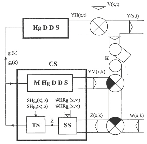
Fig. 5.3.1 DDS/PDE boundary control
| HgDDS | – controlled system with zero order holds |
| MHgDDS | – model of controlled system |
| CS | – control synthesis |
| TS/SS | – control time/space synthesis |
| K | – sampling |
| Y(x,t), YH(x,t), YM(x,k) | – distributed output variables |
| W(x,k), V(x,t) | – reference and disturbance variables |
| Z(x,k) | – modified reference variable |
| – modified lumped reference variable | |
| g1(k), g2(k) | – control variables |
In accordance with conclusions of chapter Distributed parameter open-loop control the reference variables of the SISO loops in the TS block take the forms
| (5.3.1) |
| (5.3.2) |
where ![]() are internal points from interval <0,L>.
are internal points from interval <0,L>.

Fig. 5.3.2 DDS/PDE control
| HTiDDS | – controlled system |
| MHTiDDS | – model of controlled system |
| CS | – control synthesis |
| TS/SS | – control time/space synthesis |
| K | – sampling |
| Y(x,t), YH(x,t), YM(x,k) | – distributed output variables |
| W(x,k), V(x,t) | – reference and disturbance variables |
| Z(x,k) | – modified reference variable |
| – modified lumped reference variable | |
| – vector of control variables |
Characteristics used are defined similarly as stated above:
| SHg1( SHg2( |
– lumped transfer functions between discrete boundary conditions g1(k), g2(k) and partial distributed output variables in points |
| HRg1(x,)HRg2(x,) |
– reduced steady-state distributed transient response functions to step changes of boundary conditions |
| {SHi(xi,z)}i | – transfer functions between lumped input variables |
| {HRi(x,)}i |
– reduced steady-state distributed transient response functions to step changes of lumped input variables |
Stability, performance and controllability
The dynamics of LDS under consideration is split up into time and space components. Therefore, the problems of stability and control performance has to be analysed in both, time and space domain.
In steady-state, the distributed output variable can be expressed in the form:
| (5.4.1) |
where {Yi(xi,
)}i are partial distributed output variables at points {xi}i=1,n, Y(x,) is the overall output variable and {HRi(x,)}i are HLDS’ reduced transient response functions in steady-state, see eqs.(3.1.32 – 39) and Fig. 3.1.14.
To begin, assume that individual lumped SISO control loops in the block TS are stable and {HRi(x,)}i are bounded functions, see e.g. the open control loop, Fig. 5.1.1.
Assume the distributed control loop to be in steady-state. For arbitrary, bounded step change of the distributed reference variable in the SS block, vectors of bounded lumped reference variables are got, as solutions of the approximation problem. In SISO stable loops of the TS block, the bounded values of steady-state output variables are set. For bounded functions {HRi(x,)}i also the respective output variables will be bounded in the steady-state. It means, that necessary and sufficient conditions of stability of the distributed parameter control system are determined by both, stability conditions of SISO lumped parameter control loops in the TS block and by boundedness of {HRi(x,)}i. The same bounded-input/bounded-output conclusions hold true also for closed distributed parameter control systems.
The performance of control is given in general by evolution of control error, E(x,k) = W(x,k)-Y(x,k), in a norm appropriately chosen.
In engineering practice it may be very useful to evaluate the control performance in both, time and space domain, particularly
– in the space domain
It is given by the quality of approximation of the reference variable by controlled variable in steady-state.
– in the time domain
The control performance is given by requirements put on courses of controlled variables, {Yi(xi,k)}i e.g. between particular steady-states.
In practice, the performance of control in space domain is often given by a positive real number,  , which stands for constrain of the control error quadratic norm.
Then, for a given configuration, number and forms of {HRi(x,)}i it can yield:
 |
(5.4.2) |
This means that LDS is not controllable in the space domain.
To ensure the controllability of LDS, it is necessary to find such configuration, number and forms of {HRi(x,)}i, that the following inequality holds:
 |
(5.4.3) |
The solution of this problem is subject to optimization of the distributed parameter control system.
The control performance in time domain, for variables {Yi(xi,k)}i can be ensured by appropriate choice of the SISO control loops in the TS block.
Optimization of distributed parameter control systems
When optimizing control systems, Figs. 5.1.1, 5.2.1, 5.2.2, 5.3.1, … three basic problems are to be solved. Two problems lie in the space domain, that are: minimization of the number of measuring points and minimization of the number of control variables. The third problem is related to optimization of control system performance in time domain.
– Minimization of the number of measuring points
The accuracy of approximation of the distributed output variable is given by the number and location of distributed output variable’s measuring points and by the choice of the approximation procedure (see chapters Model accuracy, Experimental identification). The control system optimization objective is, for an approximation accuracy,  ,given, to minimize the number of measuring points.
– Minimization of the number of control variables
The control performance in space domain is given by the number and the location of control members and by reduced steady-state distributed transient response functions, {HRi(x,)}i=1,n. The optimization problem aimed at minimization of the number of control variables is solved using the results of approximation theory.
– Optimization of control system operation in time domain
The dynamics of control system are determined by dynamic properties of servodrives and distributed input generators as well as by dynamic properties of the distributed-input/distributed-output system under consideration.
Optimization of control system in time domain involves the design of the SISO optimal control loops for particular control variables with respect to control performance requirements given.
| <<< Previous | Next >>> |