Distributed parameter systems can be found in various technical and non-technical branches in the form of lumped-input/distributed-output systems. In this chapter, some typical examples of real lumped-input/distributed-output systems will be shown.
Fluidized bed fireplace for high power steam generator – Fig. 2.1
By the combustion of low caloric combustibles large amount of SO2 arises. Therefore, it is necessary to maintain the temperature of the fluidized bed near optimal desulphurisation temperature. This is the task of control. Furthermore, fluctuations of heating value up to 30% have to be considered.
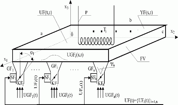
Fig. 2.1 Fluidized bed fireplace (one of the system of six fireplaces)
| FV | – fluidized bed |
| P | – high pressure part of the steam generator |
| a, b, c | – geometrical dimensions of the fireplace |
| – x1, x2, x3 | |
| {Tj}j | – thermometers |
| {GFi}i=1,n | – subsystems of pneumatic fuel and additives’ transport, generators of distributed input variables |
| {Y i}i=1,n | – output angles of pneumatic fuel and additive’s transport system |
| {SFi}i=1,n | – servodrives |
| {KFi}i=1,n | – control valves of pneumatic fuel and additives’ transport system |
| {ji}i=1,n | – valves rotation {KFi}i=1,n |
| – thermal field of FV, distributed output variable | |
| – FV resulting distributed input variable | |
| – FV distributed input variables | |
| – fuel and additive’s flow, lumped input variables for {GFi}i=1,n | |
| – vector of lumped input variables – servodrives of fluidized bed fireplace |
Now let us analyse this fluidized bed fireplace’s operation from the point of view of controlled system with lumped-input/distributed-output, Fig. 2.1.
Control variables of the control system, {UFi(t)}i=1,n, influence the actuating members of lumped input variables – servodrives {SFi}i=1,n. Their outputs appear as lumped variables – motions of valves {KFi}i=1,n : {j i}i=1,n, which determine the fuel and additives flow rates: {UGFi(t)}i=1,n.
The dynamics of the transformation between {UFi(t)}i=1,n and {UGFi(t)}i=1,n, in general the actuating members {SAi}i=1,n between control variables {Ui(s)}i=1,n and input variables {UAi(s)}i=1,n , is represented by a group of transfer functions {SAi(s)}i=1,n. Fig. 2.2.
The subsystems of pneumatic fuel and additives’ transport, {GFi}i=1,n form distributed input variables, ![]() . In general, generators of distributed input variables, {GUi}i=1,n form distributed input variables
. In general, generators of distributed input variables, {GUi}i=1,n form distributed input variables ![]() . Their dynamic properties are given by distributed transfer functions,
. Their dynamic properties are given by distributed transfer functions, ![]() , Fig. 2.2.
, Fig. 2.2.
The resulting distributed input variable,  , is acting in the input of the fluidized bed – real distributed-input/distributed-output system. As shown in Fig. 2.2, the distributed input variable,
  , is acting in the input of the distributed-input/distributed-output system, this system having the dynamics given by distributed transfer function,
 ![]() .
.
Thermal field of fluidized bed represents the distributed output variable of the fireplace, ![]() . The output variable of the lumped-input/distributed-output system, shown in Fig. 2.2, is identical with the output variable of the distributed-input/distributed-output system,
. The output variable of the lumped-input/distributed-output system, shown in Fig. 2.2, is identical with the output variable of the distributed-input/distributed-output system, ![]() .
.
Similar configuration of real distributed systems having lumped and distributed parameter elements in the structure of LDS can be found also in other technological and manufacturing processes, as described bellow.
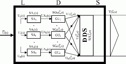
Fig. 2.2 The structure of lumped-input/distributed-output system
| LDS | – lumped-input/distributed-output system |
| {SAi}i=1,n | – actuating members of lumped input variables |
| {GUi}i=1,n | – generators of distributed input variables |
| DDS | – distributed-input/distributed-output system |
| – vector of lumped input variables of LDS | |
| {UAi(s)}i=1,n | – lumped input variables for {GUi}i |
| – DDS distributed input variables | |
| – resulting DDS distributed input variable | |
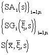 |
– transfer functions of lumped and distributed subsystems |
Rolling mill heating furnace – Fig. 2.3
Operating modes of rolling mill heating furnace are given by the technology of rolling mill. With particular operation modes, {Ti, To, Q, V, v}, particular reference values of vault temperature field YR(x,t) are associated. The control task then consists of determination of relations between vault temperature fields, YV(x,t) and YR(x,t), ensuring adequate heating of semi-products, YP(x,t), and following technological needs. Here, the controlled process dynamics exhibit time-variant, distributed and non-linear character.
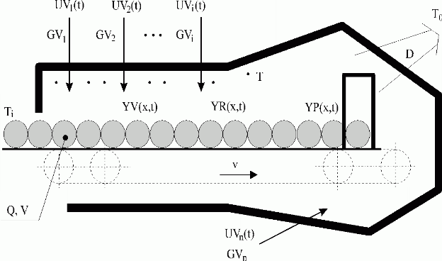
Fig. 2.3 Rolling mill heating furnace
| GVi | – i-th gas burner, generator of distributed input variable |
| T | – vault temperature thermometers |
| Q | – semi-products dimensions |
| V | – semi-products composition |
| v | – speed of semi-products shift |
| D | – transport to rolling mill train |
| Ti, To | – semi-products input/output temperatures |
| {UVi(t)}i=1,n | – gas flows, lumped input variables of {GVi}i=1,n |
| YV(x, t) | – vault temperature field, distributed controlled variable |
| YP(x, t) | – semi-products temperature field, distributed output variable |
| YR(x, t) | – reference values of vault temperature field |
High power nuclear reactor – Fig. 2.4
Nuclear reactor having the power output of about 1000 MW can be considered as time-dependent, non-linear distributed parameter system.
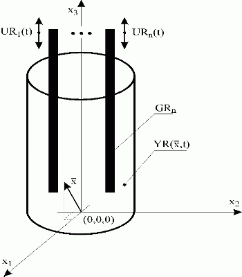
Fig. 2.4 High power nuclear reactor
| {GRi}i=1,n | – control bars, generators of distributed input variables |
| {URi(t)}i=1,n | – control bars positions, lumped input variables |
| – neutrons flow density, distributed output variable | |
| – {x1, x2, x3} |
Environmental pollution control of city agglomeration – Fig. 2.5
Maintenance of the desired quality of atmosphere composition as a distributed variable, represents very often an acute problem in densely inhabited city agglomerations.
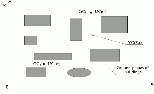
Fig. 2.5 Environmental pollution control in city agglomeration
| {GCi}i=1,n | – ejectors of oxygen, generators of distributed input variables |
| {UCi(t)}i=1,n | – oxygen flow rates, lumped input variables |
| – chemical composition of the air, distributed output variable | |
| – {x1, x2} |
Hot-house temperature field control – Fig. 2.6
Large hot-houses in agriculture and biotechnology can be also considered as typical representatives of distributed parameter systems.
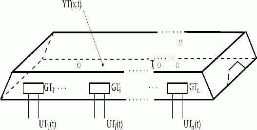
Fig. 2.6 Hot-house temperature field control
| {GTi}i=1,n | – heating bodies, generators of distributed input variables |
| {Tj}j | – thermometers |
| {UTi(t)}i=1,n | – heat flow rates, lumped input variables |
| YT(x,t) | – thermal field, distributed output variable |
Circular plate with piezoceramic patches – Fig. 2.7
Examples discussed above mostly belong to diffusion type of processes. Similar structures can be created also in oscillation type distributed systems such as control of motion in continuum mechanical systems, see Fig.2.7, [2], when measurement and control of fields of variables is realized on the basis of smart material structures, Fig.9.1.3.1, 9.1.7.1.
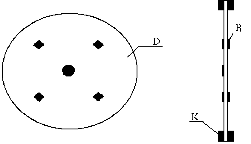
Fig. 2.7 Control of a thin circular plate with surface-mounted piezoceramic patches
| D | – thin circle plate |
| K | – bed |
| {Pi}i=i,n | – piezoceramic actuators, generators of distributed input variables |
Liver excretion process – Fig. 2.8
In the following, examples, farther from technical practice will be shown: the liver and lungs of human body. Right at identification and modeling of these organs dynamics, the structure of lumped-input/distributed-output systems was discovered.
Functions of these organs as to their input/output relations has been indicated in Introduction. When analysing the dynamics of these processes, contrast iodine compounds, radioisotopes or isotopic carriers, e.g. aerosols can be used.
First, let us consider the process of liver excretion – Fig. 2.8. The maximal size of the liver excretion system in standard (physiological) state is about 20-25 cm. The excretion process takes place in liver cellular structures. This system can be considered as a typical lumped-input/distributed-output system.
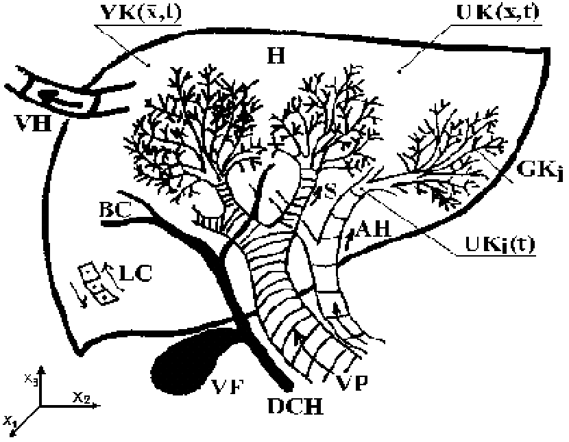
Fig. 2.8 Liver excretion process
| H | – liver |
| LC | – liver cellular structure |
| BC | – bile canaliculus |
| S | – sinusoid |
| VP | – portal vein |
| VF | – gall – bladder |
| DCH | – choledochus |
| AH | – arteria hepatica |
| VH | – hepatic vein |
| {UKi(t)}i=1,n | – contrast material flows, lumped input variables |
| – contrast material concentration in the input of excretion process | |
| – contrast material concentration in the output of excretion process | |
| {GKi}i=1,n | – anatomic parts, subsystems of liver complex’s blood and contrast material distribution, distributed input variables generators |
| – {x1, x2, x3} |
Pulmonary blood circulation – Fig. 2.9
Similar structural layout can be found also by the study of dynamics of other internal organs of the human body: kidneys, stomach or lungs – Fig. 2.9.
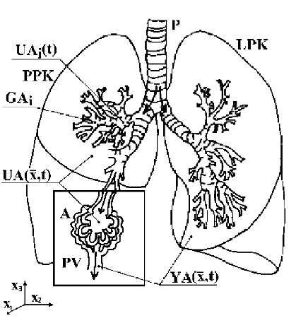
Fig. 2.9 Pulmonary blood circulation
| P | – trachea |
| PPK | – right pulmonary wing |
| LPK | – left pulmonary wing |
| A | – alveolus |
| PV | – pulmonary vein |
| {UAi(t)}i | – flows of the aerosol inhaled, input variables |
| – concentration of the aerosol in the input of the diffusion system | |
| – concentration of the aerosol in the output of the diffusion system | |
| {GAi}i | – anatomic parts, distributed input variables generators |
| – {x1, x2, x3} |
| <<< Previous | Next >>> |