Adaptive Control

On the basis of dynamics decomposition and control system design for LDS, discussed in the previous chapters, it is possible to formulate and solve various other problems of these systems control. In this chapter adaptive and predictive distributed parameter control systems will be constructed. Possible approaches to the use of classical lumped parameter systems theory results in LQG control synthesis [52, 68] and GPC of lumped parameter systems [11-13, 69, 73] will be presented too.

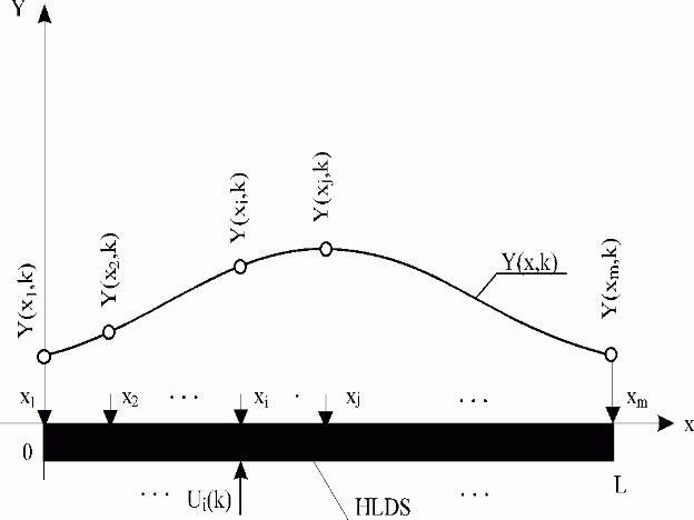
Fig. 7.1 Location of measuring points for the distributed output

HLDS	– controlled system with zero-order hold units
Ui(k)	– lumped input variable
{Y(xj,k)}j	– partial distributed output variables

Consider the system distributed on an interval <0,L> , where measuring points x = {x₁,…,x_i,…,x_j,…,x_m} are located as shown in Fig. 7.1. Between the sequence of lumped input variables, {U_i(k)}_i=1,n = U(k), and the sequence of partial distributed output variables, {Y(x_j,k)}_j=1,m = Y(x,k), in the neighbourhood of the operating point, where the dynamics of the system can be linearized, a regression model can be written in the form:

(7.1)

where na, nb, nc are orders, A_f, C_f are diagonal matrices with non-zero elements in the diagonal: {A_f(x_j)}_j=1,m, and {C_f(x_j)}_j=1,m. B_f is a matrix of the type m  n with elements {B_f(x_j, i)}_j=1,m;i=1,n. K = {K_j}_j=1,m is a vector of absolute elements and e(x, k) = {e(x_j, k)}_j=1,m is a vector of white noises with zero mean values.

Model parameter estimates [A₁, A₂,…, A_na, B₁, B₂,…, B_nb, C₁, C₂,…, C_nc, K] will be denoted as .

For the vector of discrete distributed output variables in the (k + r) step, the following relationship holds:

(7.2)

where is the vector of predicted conditional mean values of discrete distributed output variable and e(x,k+r) is the vector of white noises, r being an integer.

Now, using appropriate approximation methods – as shown in chapters Models accuracy and Experimental identification – surfaces, approximating the continuous distributed variables, can be fitted.

In the following, similarly as in numerical solutions of PDE or FEM, no difference will be made between approximated values and approximates. Hence

(7.3)

where is the distributed variable predicted at time (k + r) and e(x,k + r) is a random component of the distributed output variable.

For control synthesis purposes we will now decompose the dynamics of the system being controlled.

First, the operation state will be introduced in neighbourhood of a point k of the time coordinate for input/output variables selected. This state is given by the sequence of input variables up to step k and by the sequence of discrete output variables up to step k-1. In the next time interval, an input of constant variables, being equal to input variables at step k will be assumed. Assuming these input and output variables, we can now use deterministic components of the regression model – equation (7.1) – to predict the discrete output variables, denoted as or, in continuous case, as .

Actual state of the system in the neighbourhood of the point k represents the operation of the system under constant input variables after time k. In this state are the decomposition of dynamics and control synthesis to be carried out. Testing signals, introduced later or the control variables got by the control synthesis after time k are assumed to be in form of sequences of variables superimposed on these constant input variables.

Let us consider in the operating state specified, the influence of an appropriate testing signal, U_i(k). The overall response of the HLDS is then modelled using the regression model, eq. (7.1). The deviation of the overall response from will be denoted as . Now, choose the i-th component of this vector, representing the HLDS response to the i-th testing signal in the neighbourhood of i-th input. Another regression model, describing relations between testing signals and the respective components can be written in the form:

(7.4)

where point estimations of parameters, will be further denoted as .

If the testing signal is a unit-step, then the deviation of the total response predicted from gives , this being the transient response of HLDS predicted in the actual operating state, . A reduced form will be denoted as .

When applying this procedure to particular input variables, estimations of finite sets of , and can be obtained. At step changes of the testing input variables, the total output variable predicted will take the form:

(7.5)

where represent responses to step input variables predicted by deterministic parts of regression models (7.4) for i =1,n.

Now analyse the possibilities of minimization of the expression

(7.6)

as an objective control function. Here E denotes the value expected, ||.|| is a quadratic norm, Y(x,k+r) is the controlled variable and W(x,k+r) is the reference variable. Assume, for simplicity, reference variable being some distributed step function in an interval <k, k+r>.

Hence:

(7.7)

(7.8)

(7.9)

holding in the sense of triangle inequality. According to eq. (7.5), it can be further written:

(7.10)

(7.11)

where

(7.12)

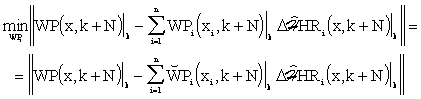
The minimization above means to minimize on the set of all output variables realizations at step k. In predictive control, however, similar problems are solved in the time domain as a sequence of optimization problems for actual variables at particular points of the time coordinate. Since E||e(x,k+r)|| has finite value at step k, then an optimization problem is to be solved only for variables of control synthesis .

Assuming step change of the distributed reference variable, by minimization of eq. (7.11) according to {WP_i }_i, lumped reference variables to control , can be obtained.

Hence:

(7.13)

Here is the vector of lumped reference variables in the operating state specified.

Now, let us design the system of predictive control with distributed parameters in terms of adaptive control, see Fig. 7.2. During the control process, is be predicted in the block PD, and at time instant k for the following cases:

A) r = N, N

B) r = N₂

then following differences are formed:

A)

(7.14)

B)

(7.15)

In the block of space synthesis, SS, the following approximation problems are solved:

A)

(7.16)

and

B)

(7.17)

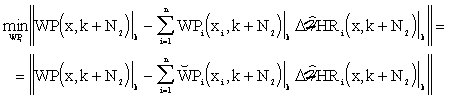
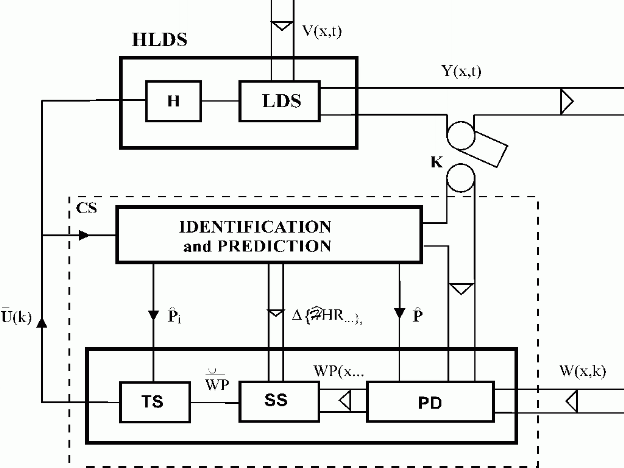
Fig. 7.2 Adaptive predictive control of distributed parameter systems

HLDS	– controlled system with zero-order hold units
CS	– control synthesis
PD	– prediction
TS/SS	– time/space synthesis
K	– sampling
	– point estimations
	– reduced distributed transient responses predicted in neighbourhood of actual operating state
	– modified reference variable
	– solution of the approximation problem, lumped reference variable
Y(x,t), W(x,k), V(x,t)	– controlled, refernce and disturbance variables
	– control variables

In the TS block, problems of control synthesis for particular reference variables, in terms of SISO control loops, are solved.

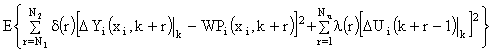
In the i-th loop, minimization of the quadratic criterion is conducted:

A)

(7.18)

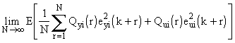
where E stands for the mean value expected, are weighting sequences. Further

and ,

where WP_i(x_i,k+r) is the reference variable converging to

When the dynamics of the i-th system being controlled is given by the regression model (7.4).

B)

(7.19)

where N₁, N₂ are minimal and maximal values of evaluating horizons, respectively, N_u is the control horizon, (r), (r) are weighting sequences and WP_i(x_i,k+r) is the sequence of reference variables, converging to

, for rN₂.

It is to notice here, that from the sequences of control increments calculated, only the first elements are applied to the process, after adding this to the previous control inputs.

In the case A), for the time rN , it yields and, following eq. (7.16), the criterion function

(7.20)

becomes minimal. Here, the control inputs are found using the LQG method of control synthesis, for each SISO predictive control loop.

In the case B), for the time r N₂ , it yields , which, in accordance with eq. (7.17), is minimizing the norm

(7.21)

through control inputs calculated by the GPC method in each particular SISO predictive control loop.

<<< Previous

Next >>>